Set environment
Code
suppressMessages (suppressWarnings (source ("../run_config_project_sing.R" )))show_env ()
You are working on        Singularity: singularity_proj_encode_fcc
BASE DIRECTORY (FD_BASE): /data/reddylab/Kuei
REPO DIRECTORY (FD_REPO): /data/reddylab/Kuei/repo
WORK DIRECTORY (FD_WORK): /data/reddylab/Kuei/work
DATA DIRECTORY (FD_DATA): /data/reddylab/Kuei/data

You are working with      ENCODE FCC
PATH OF PROJECT (FD_PRJ): /data/reddylab/Kuei/repo/Proj_ENCODE_FCC
PROJECT RESULTS (FD_RES): /data/reddylab/Kuei/repo/Proj_ENCODE_FCC/results
PROJECT SCRIPTS (FD_EXE): /data/reddylab/Kuei/repo/Proj_ENCODE_FCC/scripts
PROJECT DATA    (FD_DAT): /data/reddylab/Kuei/repo/Proj_ENCODE_FCC/data
PROJECT NOTE    (FD_NBK): /data/reddylab/Kuei/repo/Proj_ENCODE_FCC/notebooks
PROJECT DOCS    (FD_DOC): /data/reddylab/Kuei/repo/Proj_ENCODE_FCC/docs
PROJECT LOG     (FD_LOG): /data/reddylab/Kuei/repo/Proj_ENCODE_FCC/log
PROJECT REF     (FD_REF): /data/reddylab/Kuei/repo/Proj_ENCODE_FCC/references
Set global variables
Code
= "encode_open_chromatin"
Import data
Code
= TXT_REGION_FOLDER= file.path (FD_RES, "region" , txt_folder)= dir (txt_fdiry)for (txt in vec){cat (txt, " \n " )}
K562.hg38.ENCSR000EKS.ENCFF274YGF.DNase.bed.gz
K562.hg38.ENCSR000EOT.ENCFF185XRG.DNase.bed.gz
K562.hg38.ENCSR483RKN.ENCFF558BLC.ATAC.bed.gz
K562.hg38.ENCSR483RKN.ENCFF925CYR.ATAC.bed.gz
K562.hg38.ENCSR868FGK.ENCFF333TAT.ATAC.bed.gz
K562.hg38.ENCSR868FGK.ENCFF948AFM.ATAC.bed.gz
summary
Code
= TXT_REGION_FOLDER= file.path (FD_RES, "region" , txt_folder, "summary" )= dir (txt_fdiry)for (txt in vec){cat (txt, " \n " )}
description.tsv
metadata.label.tsv
Get column names
Code
### set file path = TXT_REGION_FOLDER= file.path (FD_RES, "region" , txt_folder, "summary" )= "description.tsv" = file.path (txt_fdiry, txt_fname)### read table = read_tsv (txt_fpath, show_col_types = FALSE )### assign and show = dat= dat$ Namefun_display_table (head (dat))
Chrom
Name of the chromosome
ChromStart
The starting position of the feature in the chromosome
ChromEnd
The ending position of the feature in the chromosome
Name
Name given to a region; Use '.' if no name is assigned.
Score
Indicates how dark the peak will be displayed in the browser (0-1000).
Strand
+/- to denote strand or orientation. Use '.' if no orientation is assigned.
Get metadata table
Code
### set file path = TXT_REGION_FOLDER= file.path (FD_RES, "region" , txt_folder, "summary" )= "metadata.label.tsv" = file.path (txt_fdiry, txt_fname)### read table = read_tsv (txt_fpath, show_col_types = FALSE )### assign and show = datprint (dim (dat))fun_display_table (dat)
encode_open_chromatin
K562.hg38.ENCSR000EKS.ENCFF274YGF.DNase.bed.gz
dnase_ENCFF274YGF
encode_open_chromatin
K562.hg38.ENCSR000EOT.ENCFF185XRG.DNase.bed.gz
dnase_ENCFF185XRG
encode_open_chromatin
K562.hg38.ENCSR483RKN.ENCFF558BLC.ATAC.bed.gz
atac_ENCFF558BLC
encode_open_chromatin
K562.hg38.ENCSR483RKN.ENCFF925CYR.ATAC.bed.gz
atac_ENCFF925CYR
encode_open_chromatin
K562.hg38.ENCSR868FGK.ENCFF333TAT.ATAC.bed.gz
atac_ENCFF333TAT
encode_open_chromatin
K562.hg38.ENCSR868FGK.ENCFF948AFM.ATAC.bed.gz
atac_ENCFF948AFM
Import data
Code
= function (txt_input){### setup mapping = dat_metadata= dat$ FName= dat$ Label### mapping string = fun_str_map_match (txt_input, vec1, vec2, .default= txt)= gsub ("^dnase" , "DNase" , txt_output)= gsub ("^atac" , "ATAC" , txt_output)return (txt_output)
Code
### set directory = TXT_REGION_FOLDER= file.path (FD_RES, "region" , txt_folder)= file.path (txt_fdiry, "*bed*" )### get file names and labels = Sys.glob (txt_fglob)= basename (vec_txt_fpath)= fun_str_map_file_label (vec_txt_fname)### read tables = lapply (vec_txt_fpath, function (txt_fpath){= read_tsv (txt_fpath, col_names = vec_txt_cname, show_col_types = FALSE )return (dat)names (lst) = vec_txt_label### assign and show = lstprint (length (lst))
Check data
Code
= lst_dat_import= names (lst)for (txt in vec){cat (txt, " \n " )}
DNase_ENCFF274YGF
DNase_ENCFF185XRG
ATAC_ENCFF558BLC
ATAC_ENCFF925CYR
ATAC_ENCFF333TAT
ATAC_ENCFF948AFM
Code
= lst_dat_import= lst[[1 ]]fun_display_table (head (dat, 3 ))
chr1
181400
181530
.
0
.
0.299874
-1
-1
75
chr1
778660
778800
.
0
.
14.138300
-1
-1
75
chr1
779137
779200
.
0
.
0.331440
-1
-1
75
Code
= lst_dat_import= lst[[2 ]]fun_display_table (head (dat, 3 ))
chr1
139369
139421
.
0
.
0.0872467
-1
-1
75
chr1
180800
180871
.
0
.
0.1371020
-1
-1
75
chr1
181108
181200
.
0
.
0.1246380
-1
-1
75
Code
= lst_dat_import= lst[[6 ]]fun_display_table (head (dat, 3 ))
chr1
42030
42399
.
839
.
4.94006
56.98604
54.92928
250
chr1
68963
70035
.
1000
.
3.99240
43.21727
41.22760
115
chr1
68963
70035
.
1000
.
6.60048
110.44444
108.21621
760
Explore data
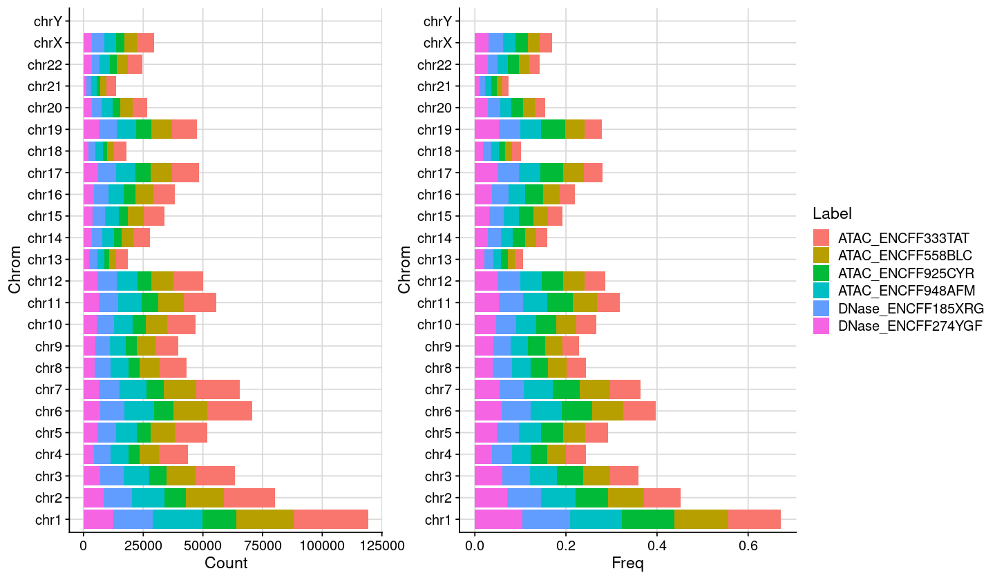
Chromosome distribution (Bar plots)
Code
### count chromosomes = lst_dat_import= lapply (lst, function (dat){= as.data.frame (table (dat$ Chrom, dnn = "Chrom" ))return (dat)### merge results = bind_rows (lst, .id = "Label" )= dat %>% tidyr:: spread (Chrom, Freq) %>% replace (is.na (.), 0 )### summarize counts to frequency = dat %>% :: gather (Chrom, Count, - Label) %>% :: group_by (Label) %>% :: mutate (Total = sum (Count)) %>% :: ungroup () %>% :: mutate (Freq = Count / Total)### assign and show = datprint (dim (dat))fun_display_table (head (dat))
ATAC_ENCFF333TAT
chr1
31171
269800
0.1155337
ATAC_ENCFF558BLC
chr1
24045
203874
0.1179405
ATAC_ENCFF925CYR
chr1
14206
123009
0.1154875
ATAC_ENCFF948AFM
chr1
20798
181340
0.1146906
DNase_ENCFF185XRG
chr1
16479
159277
0.1034613
DNase_ENCFF274YGF
chr1
12452
118721
0.1048846
Code
### set chromosome names = c (1 : 22 , "X" , "Y" )= paste0 ("chr" , vec)= vec### set factor levels = dat_stats_chrom= dat %>% dplyr:: mutate (Chrom = factor (Chrom, levels = vec_txt_chrom))### plot chromosome distribution = ggplot (dat, aes (x= Count, y = Chrom, fill= Label)) + geom_col () + theme_cowplot () + background_grid () + theme (legend.position = "none" )### plot chromosome distribution = ggplot (dat, aes (x= Freq, y = Chrom, fill= Label)) + geom_col () + theme_cowplot () + background_grid ()### combine plot = plot_grid (gp1, gp2, nrow = 1 , rel_widths = c (2 , 3.1 ))### show plot options (repr.plot.height= 7 , repr.plot.width= 12 )print (plt)
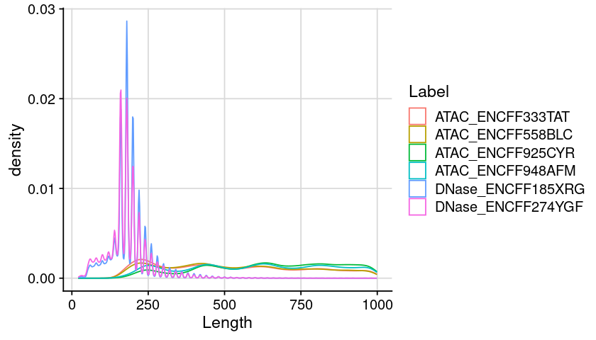
Distribution of region length (Combine)
Code
### arrange table for plot = lst_dat_import= bind_rows (lst, .id = "Label" )= dat %>% :: mutate (Length = ChromEnd - ChromStart) %>% :: filter (Length < 1000 )### create plot = ggplot (dat, aes (x = Length, color = Label)) + geom_density () + theme_cowplot () + background_grid ()### show plot options (repr.plot.height= 4 , repr.plot.width= 7 )print (gpt)
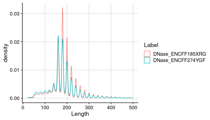
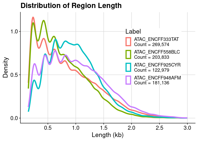
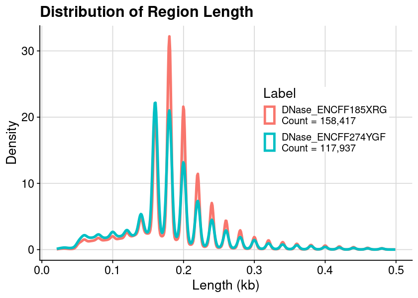
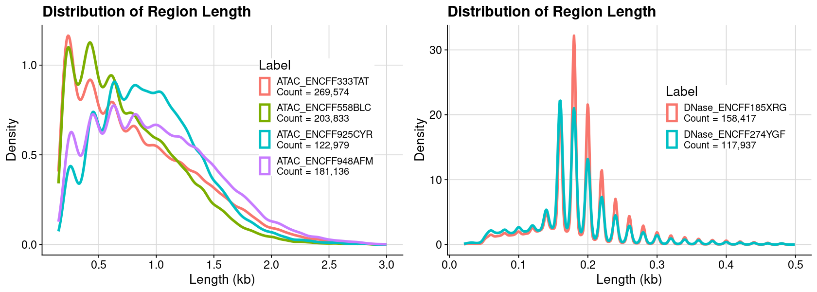
Distribution of region length (Split by ATAC and DNase)
Code
= lst_dat_import= names (lst)for (txt in vec){cat (txt, " \n " )}
DNase_ENCFF274YGF
DNase_ENCFF185XRG
ATAC_ENCFF558BLC
ATAC_ENCFF925CYR
ATAC_ENCFF333TAT
ATAC_ENCFF948AFM
Code
### split data frame into ATAC and DNase = lst_dat_import= bind_rows (lst[1 : 2 ], .id = "Label" )= bind_rows (lst[3 : 6 ], .id = "Label" )= df1 %>% dplyr:: mutate (Group = "DNase" )= df2 %>% dplyr:: mutate (Group = "ATAC" )### assign = df1= df2
Code
### arrange table for plot = dat_region_dnase= dat %>% :: mutate (Length = ChromEnd - ChromStart) %>% :: filter (Length < 500 )### create plot = ggplot (dat, aes (x = Length, color = Label)) + geom_density () + theme_cowplot () + background_grid ()### show plot options (repr.plot.height= 4 , repr.plot.width= 7 )print (gpt)
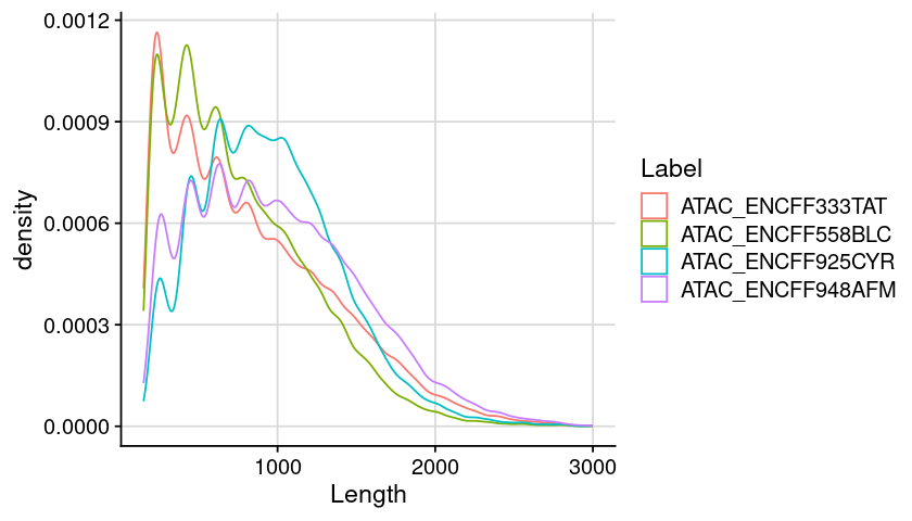
Code
### arrange table for plot = dat_region_atac= dat %>% :: mutate (Length = ChromEnd - ChromStart) %>% :: filter (Length < 3000 )### create plot = ggplot (dat, aes (x = Length, color = Label)) + geom_density () + theme_cowplot () + background_grid ()### show plot options (repr.plot.height= 4 , repr.plot.width= 7 )print (gpt)